1. INTRODUCTION

Rock discontinuities including joints, faults, or bedding planes are the weak surfaces existing in a rock mass, which can have a significant influence on the strength, deformability, and permeability of the rock mass. Understanding the discontinuity network in the rock mass is vital for the design of the tunnel as well as the safety of tunnel construction. Until now, the mapping of discontinuity has relied heavily on manual sketch at the tunnel face poses safety risks for operators working in the potentially unstable tunnel face. Additionally, the mapping results are prone to be subjective, depending on factors like measurement quantity, time constraints, and experience of the operators. These reasons highlight the need for an automatic, safer, and more objective method for mapping discontinuity in tunneling projects. Recently, the advances in 3D surface reconstruction technology such as photogrammetry or LiDAR scanning allow us to remotely create a highly accuracy 3D model of a tunnel face for further characterization of rock mass structure. The use of these techniques not only enhances the safety and efficiency of the tunnel face mapping task but also enables an automatic process to perform this task (Pham et al., 2022). In the literature, there are several automatic and semi-automatic techniques available for extracting geometrical information of discontinuities (dip and strike) based on the digital 3D models of rock faces (Lato et al., 2012, Riquelme et al., 2014). The major advantage of the automatic mapping approaches is that they can minimize bias-error induced by human interaction to provide the objective result with less time and effort. In general, the existing methods are founded on the concept of extracting planar features from unstructured 3D point clouds, as discontinuities in rock masses are often regarded as planar or nearly planar surfaces. The extraction of these planar features can be accomplished through various approaches, including region growth (Li et al., 2016), surface fitting using the Hough transform, Fourier transform (Singh et al., 2022), or random sample consensus algorithms (Kong et al., 2020) and unsupervised clustering-based methods such as the K-mean clustering algorithm (Chen et al., 2016). Although these approaches have been demonstrated successfully on ideal and simple 3D scenarios, they face difficulties when applied to complicated rock faces with high noise presence (Liu et al., 2019, Chen et al., 2023). Daghigh et al. (2022) highlight several common drawbacks associated with these mentioned methods, including their reliance on human interaction, their failure to identify discontinuity planes that are perpendicular to rock faces or only appear as traces, and their limited applicability to slightly curved surfaces. Moreover, as the limit of the principle of extracting planar features, these methods are unable to distinguish between man-made planes (e.g., those resulting from blasting or scaling processes) and actual discontinuity planes.

In this paper, we propose a new approach for automatically and accurately quantifying rock mass discontinuities based on the 3D model of the tunnel face. In general, our method is based on the principle of supervised semantic segmentation with deep learning to discriminate the areas of discontinuity from the normal areas on a tunnel face. The key idea of our approach is that the 3D model of the tunnel face will be projected into several different 2D images to identify the discontinuity areas instead of working directly on its 3D nature. These 2D images include RGB image, depth map image as well as local curvature and normal color-coded images, each contributing to a comprehensive 3D representation of the tunnel face. The combination of these different feature images can enhance the accuracy and robustness of the discontinuity detection process in 2D images. A 2D deep learning semantic segmentation model is used for segmenting discontinuity areas based on these input images. After the segmentation process, the segmentation result is projected back onto the 3D model using depth maps and projection matrices, which recover the accurate representation of the location and extent of the detected discontinuities within the 3D space. In order to demonstrate the effectiveness of our approach, we also adopted a well-known open-source software called Discontinuity Set Extractor (DSE) for comparison purposes (Riquelme et al., 2014).

2. METHODOLOGY

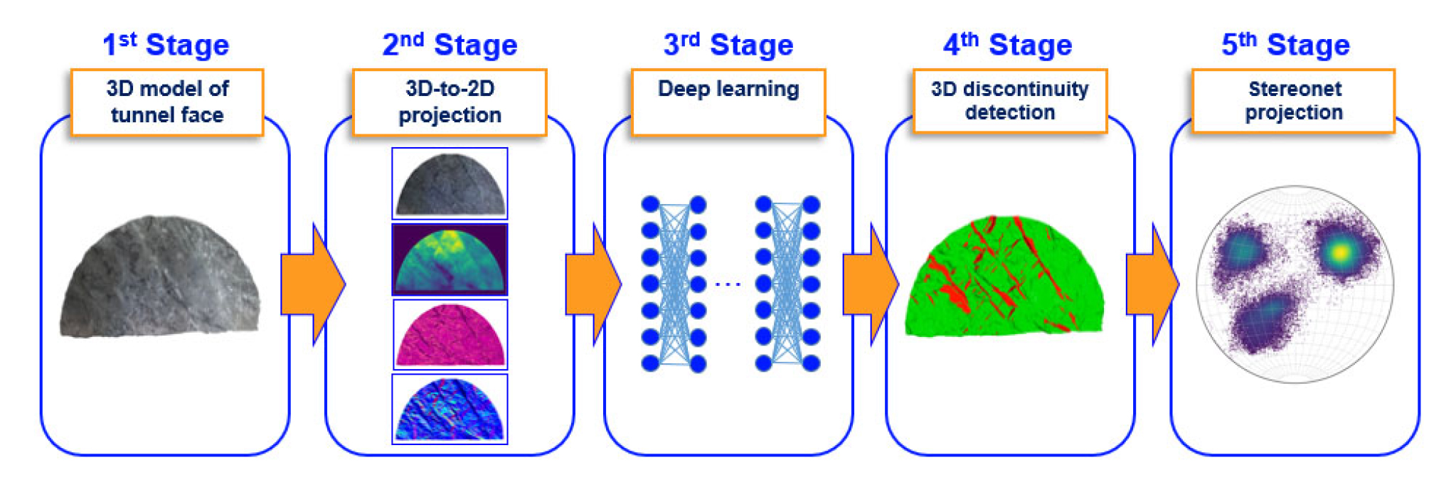
In general, our approach is composed of several major steps as follows (Fig. 1). First is the 3D-to-2D projection step, in which we generate 4 different images based on the 3D model of the tunnel face (i.e., RGB image, depth map image, local curvatures, and normal vectors color-coded images) and the labeled image obtained by projecting the corresponding manually-labeled ground truth 3D model of the tunnel face. The first four images are used as the input image, while the labeled image is used as the ground truth for training the deep learning model in the next step. Second, each set of the 2D images is subjected to pixel-wise segmentation using a fully convolutional network known as U-Net (Ronneberger et al., 2015). In the following, the segmentation result is re-projected back to the 3D space based on the depth map and projection matrices of each group to update the 3D model of the tunnel face to accurately reflect the 3D nature of the rock discontinuities identified in the 2D segmentation step. Finally, geometrical information of discontinuity planes (i.e., strikes and dips) can be obtained with the analysis of the projection of normal vectors of discontinuity points on the steoreonet. In the following, we will discuss in detail our approach from dataset preparation to the implementation and training of the deep learning model.

Fig. 1

Proposed approach for extracting rock discontinuities on a 3D model of tunnel

2.1 Dataset preparation

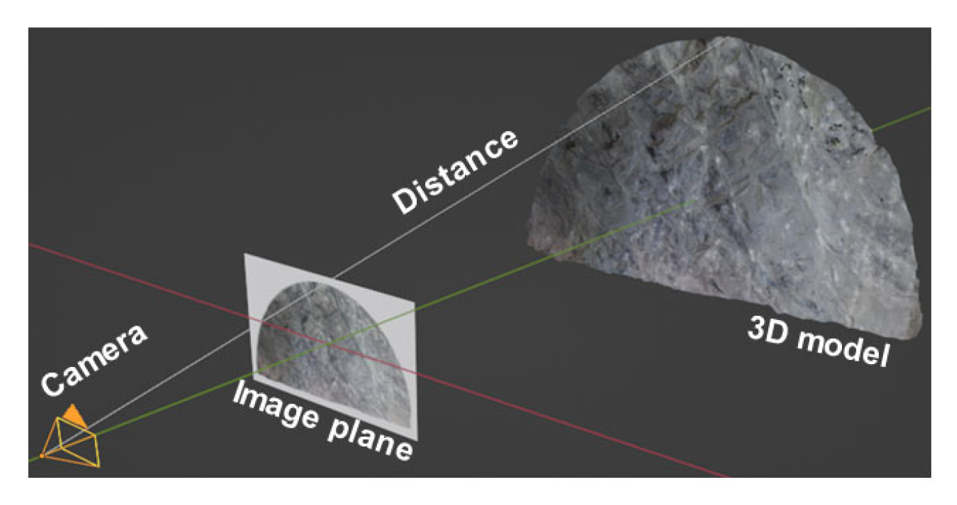
The 3D models of tunnel faces used in this study were acquired from two different tunnel projects. The cross-sections of the tunnels in the full-face excavation are approximately 80 m² with a width of ~10 m and a height of ~8 m. In total, we have 19 3D models of tunnel faces that were obtained by both LiDAR scanning (Leica BLK360 Imaging Laser Scanner) and photogrammetry techniques. Among those, 16 3D models are used for training, while the other three are kept aside for testing the deep learning model after training. The 3D models have been pre-processed using free software called MeshLab to remove noises, crop out the unnecessary parts (i.e., shotcrete-covered tunnel walls and tunnel floor), and uniformly resample the 3D mesh (Cignoni et al., 2008). As a result, we can obtain a noise-free and uniform-distributed mesh with a mean distance between vertices of approximately 0.009 m. Each tunnel face is then manually labeled using the vertex color-filling function of MeshLab to acquire the ground truth label for training. Accordingly, every point on the 3D model is assigned with red or green color, in which red denotes the discontinuity area and green denotes the non-discontinuity area. In this step, the manual mapping sketch is also used as a reference for labeling the 3D model. Following the pre-processing step, we generate the projected images of the 3D models for training the 2D semantic deep learning model. The 3D model is projected into 2D images using a method called perspective projection, which is similar to taking a photo with a camera. In general, this technique maps points on 3D mesh onto points to a virtual image plane (Fig. 2). The virtual image plane is controlled by predefined intrinsic (i.e., camera focal length and principal point) and extrinsic matrices (i.e., camera position and orientation). The virtual camera is positioned at 25 meters away from the center of the 3D tunnel face. For each tunnel face, we generate multiple projections with multiple virtual camera views by rotating the camera around the center of 3D tunnel face model keeping the distance from the camera to the center constant. This allows us to produce unlimited images for training the deep learning model.

Fig. 2

Illustration of 3D-to-2D perspective projection with a single camera view

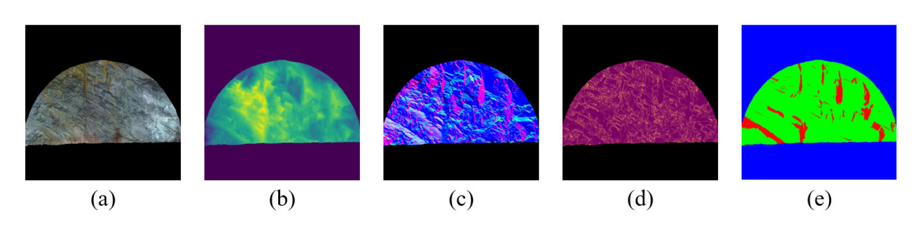
With each camera view, the abovementioned 5 images with a size of 1024×1024 pixels are obtained (Fig. 3). The four images (i.e., RGB, depth map, normal vector and curvature color-coded images) are stacked to create the input for the deep learning model (Fig. 3 (a), (b), (c), (d)). The other image (i.e., labeled images) serves as ground truth for estimating the loss value during training and evaluating the segmentation result during the testing stage (Fig. 3 (e)). The pixel values of each image are scaled to the range of 0 to 1 before feeding these images to the deep learning model. The deep learning model is trained on the projected images of the training dataset to automatically discover regularities from the input images to the semantic-labeled output image of discontinuity areas. Consequently, the trained model can be used to generate the predictions on projected images of the test dataset. The prediction results are then compared with the corresponding ground truths or labeled images to evaluate the performance of the model on previously unseen data.

Fig. 3

Example of projected images from a camera view: (a) RGB; (b) depth map; (c) normal vector color-coded; (d) curvature color-coded and (e) labeled images

2.2 Deep learning model

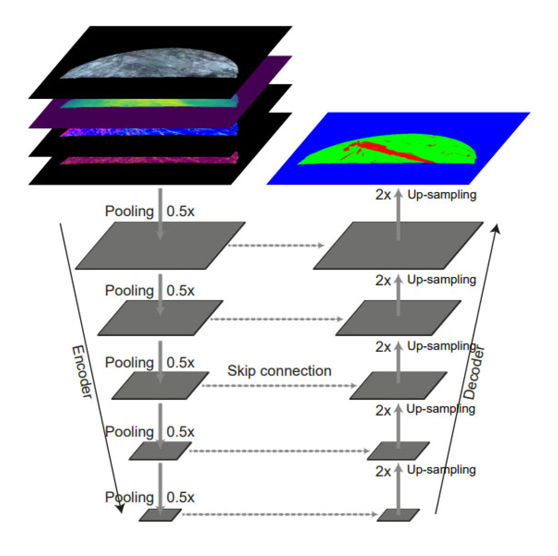
We adopted the most well-known deep learning semantic segmentation model called U-Net to automatically identify discontinuity areas based on projected images of tunnel faces. This deep learning model was first proposed in the field of biomedical image segmentation. The architecture of U-Net is basically composed of an encoder and a decoder, which are connected by multiple-level skip connections (Fig. 4). In the encoder, the input images are passed through a sequence of convolutional and pooling layers, which progressively reduce the spatial dimensions of the input images while extracting higher-order features. The decoder is responsible for generating a prediction output from the features extracted by the encoder. It usually involves up-sampling and deconvolution layers to transform the abstract features back into a spatial representation that matches the original input image size. The network also integrates low-level and high-level features during the prediction phase by using skip connections, which fuse the feature maps from the encoder to the equivalent layers in the decoder. By combining features from different levels, the network can learn to recognize both local and global patterns, contributing to the model's ability to identify complex structures. In this study, we replace the conventional encoder with an ultra-deep network called ResNet101. Additionally, several minor changes have been made in order to match with the input and output image dimensions in our case. The U-Net model is fed with a 10-channel image that is the concatenation of four aforementioned projected images (RGB, depth map, curvature, and normal). The output of the model is an RGB image, in which red, green, and blue channels represent three classes i.e., the discontinuity area, normal tunnel face, and the background, respectively. For pixel-wise multiple-class classification, the softmax activation function is also applied to the output layer. The purpose of this activation function is to normalize the values across the channels within each pixel of the output image, yielding a probability vector where the sum of all components equals one. As a result, the label of a pixel will be assigned to the class with the highest probability.

Fig. 4

General architecture of U-Net

Since the area of discontinuity is quite small in the image compared to other classes, we decided to use a combining loss function, which is a sum of two different loss functions i.e., Categorical cross-entropy loss and Dice loss. The use of this kind of loss significantly mitigates the issue of class imbalance and also improves the performance of the segmentation model. Furthermore, a greater class weight is also assigned to the discontinuity class (i.e., red channel), allowing the model to pay more attention to this class while lowering bias towards the other two classes (i.e., green and blue channels). To assess the performance of the deep learning model, we employ the intersection-over-union (IoU) metric, which measures the similarity between the predicted segmentation result and its corresponding ground truth. The IoU score is calculated by dividing the number of the pixels common between the ground truth and the predicted result by the total number of pixels present across both. This score is calculated for each class separately and then averaged over all classes to provide a mean IoU score (mIoU) of our semantic segmentation prediction. The mIoU score is ranging from 0 to 1, such that a higher mIoU score indicates better segmentation performance. The Adam optimizer was chosen as the optimization algorithm for training the deep learning model, with an initial learning rate of = 0.0001 and a drop factor of 0.1 (Kingma and Ba, 2014). The training was performed for 200 epochs with a batch size of 2. The early stopping technique is also used to end the training if the validation mIoU does not increase after 20 epochs.

3. RESULT AND DISCUSSION

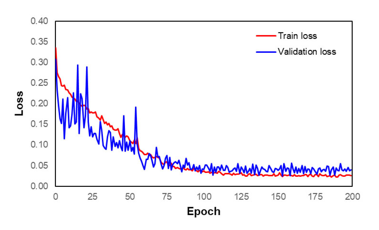
The training curves of the U-Net model are shown in Fig. 5. As we can see, both training and validation loss gradually decreases with the progress of training. This generally indicates the positive performance of the model on both the training data and unseen (validation) data. The loss curves start to converge roughly at the epoch of 150, which suggests that the model has learned as much as it can from the available data. Therefore, further training is not needed since it does not contribute to the performance of the U-Net model.

Fig. 5

Training curves: training loss (red curve) and validation loss (blue curve)

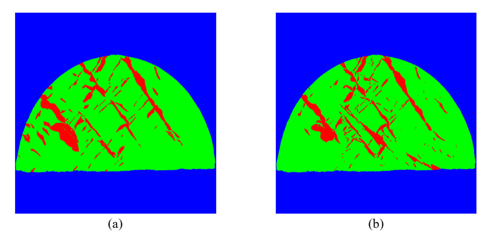
Following the training of the U-Net model, we carry out the prediction on the test images for evaluating the trained model. Fig. 6 depicts an example of the segmentation result accompanied by its corresponding ground truth. This ground truth image was obtained by projecting the manually labeled 3D tunnel face model to the same 2D image plane as the input image. Overall, the U-Net model exhibits the capability to identify discontinuity areas, achieving an average intersection-over-union (IoU) rate of approximately 0.8 on the test dataset. While the segmentation accuracy measured by IoU is promising, it remains somewhat limited, which is possibly due to the scarcity of training data. As a result, the performance of the segmentation model could be enhanced to more precisely and thoroughly detect the locations and extensions of rock discontinuities on the 3D tunnel face as the training data increases.

Fig. 6

Example of segmentation result (b) with its corresponding ground truth (a)

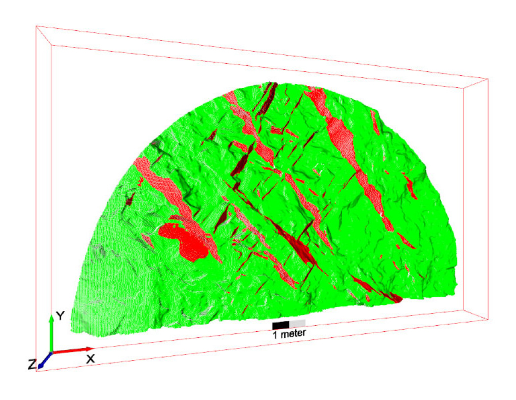
The predicted segmentation results are subsequently re-projected onto the 3D model to obtain the semantic segmentation of discontinuities in the 3D context (Fig. 7). Following the re-projection, the normal vectors of points classified as discontinuities are extracted and projected onto a stereonet for further geometrical analysis of discontinuity.

Fig. 7

3D segmented point cloud of a tunnel face obtained by re-projecting 2D segmented images to 3D space

We also adopted a program so-called DSE for extracting discontinuity on a 3D tunnel face for comparison study to demonstrate the effectiveness of our methodology. The DSE is an open-source MATLAB program, which is developed based on a semi-automatic approach proposed by Riquelme et al. (2014) for identifying planar discontinuities from a 3D point cloud of rock face. This approach begins with the estimation of the normal vector at each point on the point cloud using the k-nearest neighbor algorithm. The normal vectors of all points are then projected onto a stereonet for statistical analysis. The poles, representing general normal vectors of discontinuity sets, are automatically assigned to high-density spots on the stereonet, with the option for manual adjustments. Subsequently, an angle threshold is applied to determine if a point belongs to a discontinuity set based on the difference angle with a pole. Finally, in the post-processing step, discontinuity sets with less than ten points are eliminated, ensuring a more robust and accurate outcome.

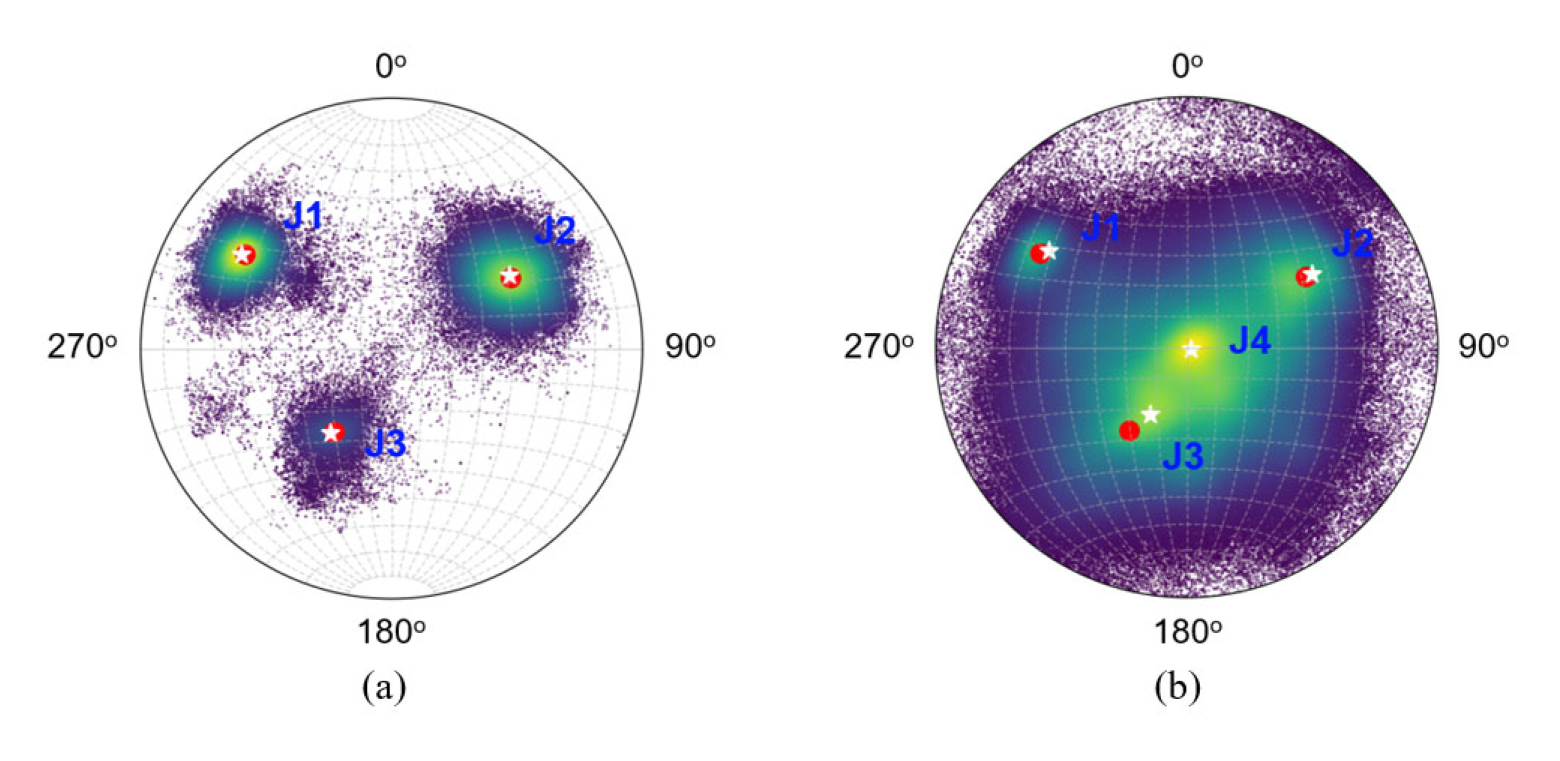
In comparison with the stereonet obtained by the DSE approach (Fig. 8 (b)), the stereonet obtained by our method shows a clear separation of the different discontinuity sets (Fig. 8 (a)). The result shows that there are three density maxima on the stereonet representing three different discontinuity sets (denoted as red dots), which is comparable to the result of manual mapping (denoted as white stars) (Fig. 8 (a)). The result obtained with DSE software also shows agreement with our approach on these three discontinuity sets (i.e., J1, J2, and J3). However, it is observed that the DSE software has detected there is another joint set that falls on the center of the conventional stereonet (i.e., J4) (Fig. 8 (b)). With such dip and strike, this joint set is actually the vertical tunnel face, which is a result of the blasting process. Additionally, it is apparent that our approach's results are more accurate than those from DSE when compared to ground truth obtained from the manual labeling result (Table 1). The discrepancy between strike/dip values obtained by our approach and the manually labeled ground truth is always less than those obtained by the DSE program.

Fig. 8

Density-colored stereonets: (a) stereonet obtained from our approach with points classified as discontinuity and (b) stereonet with all points on the 3D model (DSE)

4. CONCLUSION

This study demonstrates that our proposed approach can outperform the existing conventional approaches on rock discontinuity identification in a 3D model of the tunnel face. Despite the limitations of the training data, our approach achieves an encouraging result on discontinuity detection with an IoU score of up to approximately 0.8 on the projected images of the test dataset. Furthermore, the geometrical analysis indicates that the orientation of discontinuities obtained by our method also shows a better agreement with the manual labeling result compared with the result of the DSE method. By leveraging the benefits of a supervised machine learning approach and utilizing a combination of multiple features as input, our method offers a more reliable and efficient approach to extracting rock discontinuities on a 3D model of a tunnel face or rock face. It holds the potential to surpass existing planar feature-based methods, which depend solely on normal vectors and unsupervised machine learning algorithms for grouping points in the 3D model into distinct sets of discontinuities. Our method not only provides a new approach for automatically and accurately mapping discontinuities on a tunnel face but also significantly reduces the bias error, and the time and effort required for discontinuity mapping tasks. Additionally, this automatic mapping method can be incorporated into real-time monitoring systems, allowing for continuous tracking of changes in discontinuity patterns during tunnel excavation. This information is crucial for identifying potential stability issues, making faster decisions, and mitigating risks during tunnel construction. Furthermore, the suggested approach can extend its applicability to rock type classification and other structure detection tasks by considering all factors, including color and geometric features of the 3D model. Ongoing research efforts are essential to tackle the remaining challenges, such as limitations in training data, and to optimize the proposed approach for enhanced performance.