1. INTRODUCTION

Fractures are common structural features encountered in rocks. The characteristics and distribution of fractures can have significant effect on deformability and permeability of rock mass. In many recent applications of rock engineering such as CO₂ storage, geothermal production and nuclear waste disposal, the knowledge of fracture geometry is critical to understand the initiation and development of damage zone in response to those operations. With the advantage as non-destructive testing method, computed tomography (CT) scan recently emerged as an effective tool for geological material research (Ketcham and Carlson, 2001, Andrä et al., 2013). Many published studies demonstrate the use of CT scan to evaluating internal structure of rock sample like pore, mineral and also fracture (Wennberg et al., 2009, Kyle and Ketcham, 2015, Schmitt et al., 2016).

The fundamental step to obtain the geometric information from CT scan images is the segmentation of the feature of interest, i.e., fracture in the context of this study. In this step, fractures are detected and delineated either manually or automatically. While the manual approach is time-consuming and user-bias, the automatic is still far behind expectation. Automatic thresholding methods such as Otsu’s or Yen’s method (Yen, 1970, Otsu, 1979) are extensively used for CT scan image segmentation, which are relied on identification of a single grayscale value to partition fractures from the background. However, these methods severely suffer from the complexity of uninterested background, where the existence of non-fracture objects with similar grayscale to the one of fracture. To partly deal with this problem, ridge filters such as Hessian or Frangi filter are commonly adopted to enhance the contrast between fracture and background (Voorn et al., 2013). The major drawback of these filters is that it amplifies not only the contrast of fracture, but also mineral boundaries in the background. Thus, after thresholding step, additional attempt is always required to remove noises caused by unintended objects.

For the past few years, there has been a rapid rise in the application of deep learning in image segmentation. Various algorithms were investigated to detect and segment the fracture and crack in images including U-Net and Mask Region-based Convolutional Neural Networks (Mask R-CNN) (Ronneberger et al., 2015, He et al., 2017). In comparison with traditional approach, the deep learning algorithms are not only more effective, but also give the better results. U-Net is the most commonly used algorithm for the task of segmentation, which is simple and yields reasonable result. However, the main challenge facing this algorithm is the complexity in background and vagueness of fracture, which may lead to missing as well as mistaken detections. For Mask R-CNN, although the Mask R-CNN is considered the most effective way to obtain instance segmentation, many latest research in CT scan image segmentation indicate that Mask R-CNN works well to find bounding boxes for interested object, but its performance on segmentation is worse than U-Net. To this end, we can conclude that detection and segmentation of fracture in CT scan images in practice still remains as a very challenging task and there is still plenty of room for improvement.

In this study, we aim to develop a new approach to automatically and accurately detect fractures in CT scan images. The proposed approach is developed on the basis of Faster R-CNN algorithm with a major modification for the task of rotated bounding box prediction (Ren et al., 2015). The use of rotated bounding box for object detection has been introduced in the past few years primarily for scene text detection and ships, aircraft and other vehicles detection in aerial images. This type of bounding box have advantages over other axis-align bounding box as it allows a better spatial constrain, such that the object is unique and fully contained in the bounding box. The idea underlying our approach is to take this advantage of rotated bounding box to minimize the ratio of background within the box and consequently provide a better prior spatial information to guide the segmentation process.

2. METHODOLOGY

2.1 Rotated bounding box Faster R-CNN

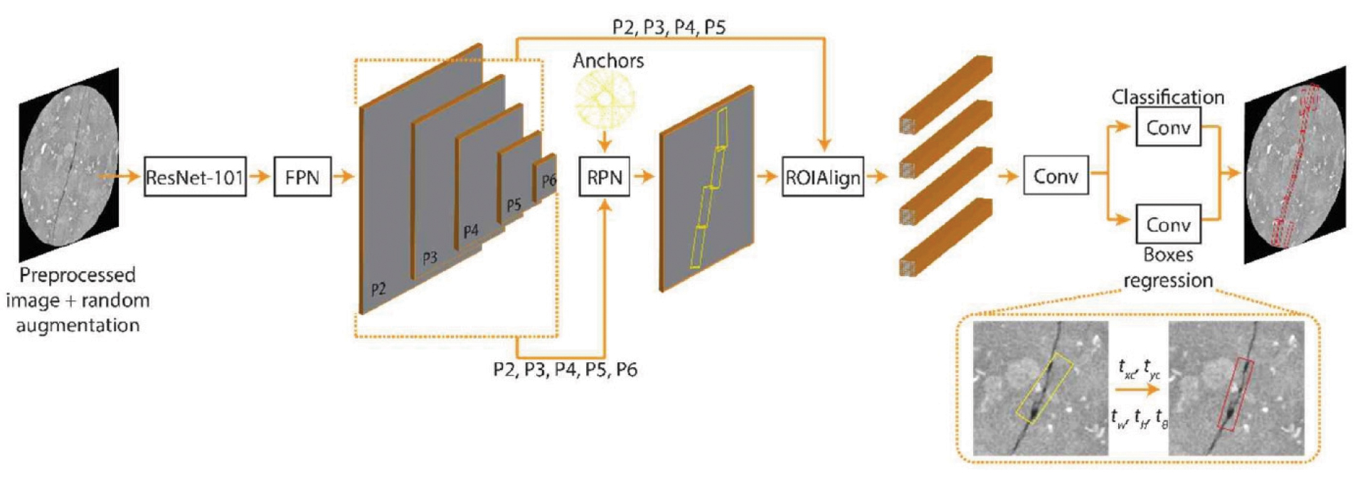
Faster R-CNN, a well-known object detection algorithm in the family of region-based algorithm, was first published in 2015 (Ren et al., 2015). Up to now, although several different models have been proposed with the aim of further improving detection performance such as You Only Look Once algorithm (YOLO) (Redmon et al., 2016) or Single Shot MultiBox Detector algorithm (SSD) (Liu et al., 2016), Faster R-CNN still remains as an outperforming algorithm in terms of detection accuracy. Despite the complexity in architecture, Faster R-CNN can be generally divided into two main components, i.e., region proposal network (RPN) and R-CNN corresponding to double stages of detection framework (Fig. 1). Apart from those two components, Faster R-CNN also adopts a deep CNN known as backbone network to extract the feature maps from input image. As usual, we use ResNet-101 in combination with Feature Pyramid Network (FPN) to obtain multi-scale feature maps (Lin et al., 2017). Loosely speaking, RPN and R-CNN perform almost similar functions but in some different fashion, including: (1) predicting bounding boxes where fracture is likely to exist and (2) refining the coordinate of those boxes to better match with the shape of fracture. The difference between them is that while RPN uses the whole feature maps extracted from input image for bounding box prediction, RCNN only takes a specific number of partial regions in the feature maps corresponding to proposal boxes (i.e., RPN’s output) and uses them for final bounding box prediction. In the following, we will discuss on the modifications within each component that are required for the purpose of rotated bounding box prediction.

Fig. 1

Rotated Faster R-CNN architecture

It is beneficial to enumerate the means of rotated bounding box and anchor box before getting into the detail of Faster R-CNN. As mentioned earlier, the detection of fracture will be in form of oriented rectangular boxes. For such bounding box representation, besides four conventional parameters, i.e., center point coordinate (xc, yc), width (w) and height (h), an additional parameter of angle (θ) is introduced to take account of box orientation. This angle is given as an angle between positive vertical axis and the longer side of bounding box, such that ranging from -90° to 90°. It is also worth to mention that the width of bounding box is always less than height. In line with rotated bounding box, anchor boxes are a set of predefined rotated bounding boxes with a certain scale, aspect ratio and angle. They are uniformly distributed over the image and will play a role as references for generating proposal boxes in RPN stage.

In short, RPN network will learn to identify anchor boxes which may contain fracture and produce target regression coefficients to convert the anchor boxes into a better proposal bounding boxes. For that purpose, RPN network is designed with a convolution layer followed by two sibling fully connected branches so-called classifier and regressor. During training, based on the overlap with ground truth boxes and predefined thresholds, the anchor boxes will be classified into 3 groups labeling as positive, negative and neutral corresponding to foreground (i.e., fracture-contained) boxes, background boxes and ambiguous boxes. Consequently, the classifier branch will learn how to predict anchor box label by using soft-max activation function. The output of this branch will be objectiveness scores, which reflect how confident the network is that a proposal bounding box contains the fracture. At the same time, one or more than one positive anchor boxes will be assigned to each specific ground truth box. The offset value between assigned anchor boxes and the ground truth box will be calculated as the equations (1) – (5) below. First four equations present the scale invariant translation between center coordinates and the log-space height-width shift. Additionally, the fifth equation presents the rotation angle in radian orientations. The regressor branch will learn to predict those offset values. Afterward, the predicted offset values will be used to transform an anchor box to the final predicted proposals via equations, which are simply the reverses of the equations (1) - (5).

where x_a, y_a, w_a, h_a and θa are x-, y-center coordinate, width, height and orientation of anchor box, respectively.

Through inspection of the result from the first training, we found a problem with using IoU (i.e., Intersection-over-Union, which is an index to measure the overlap between two boxes) for anchor box assignment. Without considering the difference in angle between two boxes, an anchor box, which has a large different angle to ground truth box, still can be assigned as positive anchor because its overlap with ground truth anchor is higher than assignment threshold. To solve this issue, we modified the conventional IoU by multiplying it with an index referred as weight of the parameter “angle” and then used this new IoU for anchor assignment. This implementation helps to decay IoU with respect to the angle difference with Gaussian penalty function as the following equation:

where Δθ is the acute angle between two oriented bounding boxes ranging from 0° to 90° and α is empirical constant (equal to 0.1 in this study).

As mentioned earlier, a ground truth box can be matched up with one or more than one anchor box. This will cause a problem that the prediction may be composed of overlapping boxes. To remove redundant boxes, the proposal boxes will be passed through a filter algorithm known as rotated non-maximum suppression (NMS). NMS will keep or remove boxes according to their objectiveness scores and IoU index, such that if a bounding box overlaps considerably with a higher objectiveness scores bounding box (i.e., IoU > 0.7), it will be removed.

However, although RPN has a bounding box regression branch, it only gives coarse bounding boxes that may contain fracture. The primary reason is due to the fact that RPN has to use high-variance anchor boxes to predict the potential boxes (Vu et al., 2019). Thus, a second stage R-CNN is needed to further refine the bounding boxes. In this stage, proposal boxes will now serve as reference boxes and also as basis to crop feature maps for the input of this stage. Since the size of the proposal boxes is different, cropped feature maps cannot be directly input into R-CNN. ROI align is therefore carried out to extract fixed size feature maps. The remaining operations within this stage is similar to RPN as described above. The outputs of R-CNN will be a list of bounding boxes along with their objectiveness scores, which is again filtered by using NMS to get the final list of predicted bounding boxes.

Faster R-CNN is optimized for a multi-task loss function, which is a combination of classification loss and box regression loss. For each region of interest, the loss function was calculated as follows:

where class_loss and box_loss represent the classification loss and bounding box regression loss in each stage (i.e., RPN and R-CNN), respectively. The bounding box regression loss for all rotated bounding box representations adopted the smooth L1 loss function, which is defined in Girshick (2015). In short, smooth L1 loss function, also known as Huber loss function, is a combination of mean square error loss and mean absolute error loss in which the square term will be used if absolute error falls below 1 and absolute term otherwise.

2.2 Experiment

To assess the performance of the proposed methods, we conducted experiments using the CT scan image dataset acquired from scanning of artificially fractured rock samples (including granite, sandstone and shale). Each of scanning provides a stack of 1024 image slices with a size of 1024 × 1024. In general, CT scan images are visualized in grayscale with value ranging from 0 to 255, which depicts X-ray attenuation coefficient of material making up the rock. The fractures appear in the images as dark and arbitrarily-oriented curved line structures with varied thickness along their length. In the initialization stage, the grayscale images undergo preprocessing in order to remove noise and to enhance the contrast between phases in CT scan images by using non-local means filter and contrast limited adaptive histogram equalization.

In total, 680 images were randomly selected from the previous sets. These images were first cropped to remove the unwanted black background. Afterward, ‘roLabelImg’, a graphical image annotation tool, is used to annotate fracture with rotated bounding boxes in those CT images. In accordance with elongated shape of fracture, we annotated fractures with head-to-tail overlapping boxes in order to avoid excessively large uninterested background included in the bounding boxes. Then, we randomly divided the dataset into train, test, and validation sets with the ratio of 7:2:1. Moreover, all the images were resized to a relatively lower resolution of 640 × 640 to obtain the same size image for model’s input as well as speed up the training and evaluation. Also, different data augmentation methods, including rotation, flip, brightness and contrast shift and sharpness, were also applied to training set to obtain more diverse CT scan images for training. This strategy is important to prevent an overfitting problem in deep learning and improve generalization performance of the model.

The algorithms presented in this study were implemented in Python using Tensorflow library (Abadi et al., 2015). We carried out experiments on a 4-core Intel Core i7-6700K @ 4.00 GHz processor with Nvidia Geforce GTX 1080 Ti GPU with 11 GB of memory. Since there were no available pre-trained weights for CT scan images, the training was performed from scratch by initializing each layer’s weights using initialization method described in He el al. (2015). The network was trained for 100 epochs using Adam optimizer with constant learning rate of 0.0001 and batch size of 2.

Finally, the mean average precision (mAP) with the IoU threshold of 0.5 was used for quantitative evaluations of our proposal method (Lin et al., 2014). Since fracture was annotated with a group of consecutive boxes instead of a large one, in many cases predicted bounding box group is mismatched with the ground truth due to the difference in individual box size and number of boxes, but the boxes still catch the same detection area. Therefore, a new reasonable box matching rule is needed to avoid underestimation of the new algorithm operation. In this study, besides using IoU as a criterion to decide whether a predicted box is true positive or false positive, we also considered the orientation of the predicted bounding box in regard to ground truth bounding boxes and number of ground truth bounding box overlapped it. Accordingly, there are two cases that a predicted bounding box can be defined as true positive prediction: (1) the predicted bounding box has an IoU higher than 0.5; and (2) the bounding box overlaps with more than two ground truth bounding boxes, and the orientation angle difference between the predicted bounding box and the ground truth boxes is less than 10 degree.

3. FRACTURE DETECTION RESULT

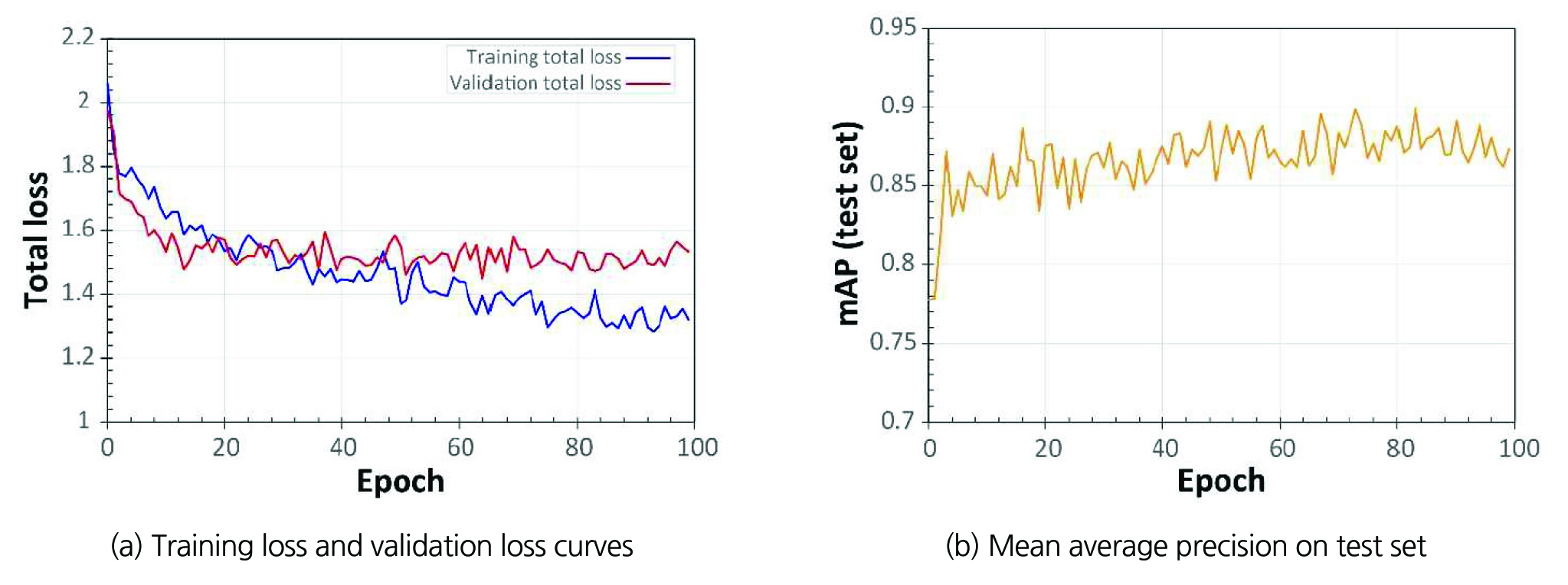
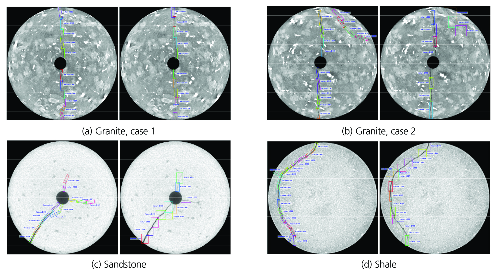
In order to ensure that the model was properly trained, we first examine the training curves. In overall, both training and validation loss curves show decreasing trends as training progressed, which means that our model performs well on unseen dataset (Fig. 2(a)). Also, we can see that the training and validation loss starts to converge after more or less 90 epochs.Thus, further training is not needed as it will not contribute to performance of the model. Besides, the model is also evaluated at the end of each epoch by calculating mAP of the model on the test dataset which is not seen in training. In Fig. 2(b), mAP versus epoch is depicted, showing that as the number of epoch increases, the mAP (accuracy) on the test dataset also increases. The model achieves its best mAP of approximately 89% on the test dataset. We also make a comparison between rotated and horizontal bounding box approaches. Both methods were trained and tested on the same dataset. Several qualitative results are shown in Fig. 3. In general, the two methods present similar performance in terms of mAP. For training and inference speed, axis-align bounding box is certainly faster than rotated bounding box approach. This is due to both facts that the number of anchor boxes in axis-align bounding box approach is much less than rotated bounding box, and IoU estimation in rotated bounding box is far more complicated and requires more computing time than in axis-align bounding box. However, the rotated bounding box approach is able to achieve more accurate detection on fractures employing less background area, which is an important factor for accurate segmentation.

Fig. 2

Training results

Fig. 3

Comparison of inference results on test image set empolying rotated (left) and horizontal (right) bounding box in each subfigure

4. DISCUSSION

In overall, we have demonstrated that our newly developed algorithm can produce reasonable results on fracture detection regardless of heterogeneity in background of CT scan image and variation in fracture size and pattern. Besides, our approach with use of axis-align bounding box has some essential advantages over the conventional approach. First, the use of rotated bounding box can effectively eliminate the background from bounding box, such that setting more robust basement for fracture segmentation. Second, it is possible to extract information on fracture length and orientation from rotated bounding box without further implementing segmentation step. To some extent, this approach is also applicable for cracks or fractures detection on buildings, roads, tunnels and other structures.

However, there still remains several limitations in the proposed algorithm. One limiting case could be where CT images are highly degraded due to artifacts, or where the fracture is too thin and is below the resolution of CT scan image. By examination of the detection result on test dataset, we noticed that most of false negative (i.e., missing detection) is related to the poor quality of these particular CT images. In such cases, CT images are highly deteriorated by artifacts including beam hardening causing dark streak overlapping fracture area and partial volume artifact causing blurriness of the fracture. However, previous research demonstrate that fluid flow in fractured porous media is mainly governed by large-aperture fractures and less tortuous fractures rather than minor fractures which have a smaller aperture and are highly tortuous (Kling et al., 2016, Crandall et al., 2017). Thus, the missing of minor fractures can be neglected without significant consequence on the characterization of fluid flow through fracture. Another limitation of this algorithm is that its training and inference speed. While the original implementation of Faster R-CNN with axis-align bounding box only uses 9 cases of anchor box (i.e., 3 scales × 3 aspect ratios), in the new approach the total case of anchor box is much higher because of one additional parameter (i.e., angle). Therefore, the effects of anchor box selection should be analyzed to obtain acceptable trade-offs between analysis speed and accuracy.

Our future efforts will be directed to explore potential ways to segment the fracture within the bounding boxes. In the end, a user interface, in which the detection algorithm is integrated seamlessly with segmentation algorithm, will be established to obtain final segmentation of fractures.

5. CONCLUSION

We present a new algorithm that is a modification based on the Faster R-CNN for fracture detection in CT scan images. Due to the complexity of uninterested background and tortuous fracture, we adopted the rotated bounding box to enhance the capability of bounding box to fit with the pattern of fracture. The experimental results show that the algorithm can accurately detect fracture and considerably reduce ratio of background in the bounding box. Although the proposed method requires some increments in the computational complexity due to the deep learning architectures, it is expected to make the fracture segmentation more accurate.